Kernel ridge regression

最小二乘，岭回归，高斯过程回归，分别是什么。

矩阵求导规则：

矩阵各种运算规则

$$\begin{aligned} Y& =A * X \quad \frac{\mathrm{d} Y}{\mathrm{d} X}=A^{T}\\ Y &=X * A \quad \frac{\mathrm{d} Y}{\mathrm{d} X}=A \\ Y& =A X B \quad \frac{\mathrm{d} Y}{\mathrm{d} X}=A^{T} B^{T} \\ Y& =A X^{T} B \quad \frac{\mathrm{d} Y}{\mathrm{d} X}=B A \\ \frac{\mathrm{d}\left(X^{T} A X\right)}{\mathrm{d} x}&=\frac{\mathrm{d} X^{T}}{\mathrm{d} x} A X+\frac{\mathrm{d} A X}{\mathrm{d} x}\left(X^{T}\right)^{T}=A X+A^{T} X \end{aligned}$$

线性最小二乘回归

线性最小二乘问题其实就是求解一组$\theta$，此时的代价函数为：

$$\begin{aligned} J(\theta) & =\frac{1}{2 m} \sum_{i=1}^{m}\left(x_{i}\theta-y_{i}\right)^{2} + \lambda\|\theta\|^{2}\\ \frac{d J}{d\theta}& =\frac{d(X \theta-y)^{T}(X \theta-y)+\lambda\theta^{T}\theta}{d \theta} \\ &=\frac{d\left(\theta^{T} X^{T}X \theta-y^{T} X y-\theta^{T} X^{T} y+y^{T} y +\lambda\theta^{T}\theta\right)}{d \theta} \\ & =X^{T} X \theta+x^{T} X \theta-X^{T} y-X^{T} y+2\lambda\theta =0 \end{aligned} \tag{2}$$ $$\begin{aligned} &X^{\top} X \theta-X^{T} y+\lambda\theta =0 \\ &X^{T} X \theta +\lambda\theta =X^{T} y \\ &\theta =\left(X^{T} X + \lambda I\right)^{-1} X^{T} y \end{aligned}$$

核岭回归

首先有：

$$\left(X^{T} X+\lambda I\right) X^{T}=X^{T} X X^{T}+\lambda X^{T}=X^{T}\left(X X^{T}+\lambda I\right)$$

这个式子左乘$\left(X^{T} X+\lambda I\right)^{-1}$并右乘$\left(X^{T} X+\lambda I\right)^{-1} X^{T} y$可以得到：

$$X^{T}\left(X X^{T}+\lambda I\right)^{-1} y=\left(X^{T} X+\lambda I\right)^{-1} X^{T} y$$

其中右边即为$ \theta$:

$$X^{T}\left(X X^{T}+\lambda I\right)^{-1} y=\theta \tag{3}$$

【其实上式可以根据式（2）推导】
令：

$$\alpha=\left(X X^{T}+\lambda I\right)^{-1} y$$

则有：

$$\theta=X^{T} \alpha$$

对于一个新的观测值$\left(x^{\prime}, y^{\prime}\right)$
如果【其中$x^{\prime}$是行向量】，那么预测值为：

$$\hat{y}^{\prime}=x^{\prime}\theta=x^{\prime}X^{T}\left(X X^{T}+\lambda I\right)^{-1} y$$

如果【其中$x^{\prime}$是列向量】，那么预测值为：

$$\hat{y}^{\prime}=\theta^{T} x^{\prime}=y^{T}\left(X X^{T}+\lambda I\right)^{-1} X x^{\prime}$$

设：

$$K_{i j}=x_{i} x_{j}^{T}$$ $$\kappa_{i}=x_{i} x^{\prime}$$

其中$x_{i}$是矩阵$X$的一个行向量，也就是一个样本。此时$K$是核矩阵，其每个元素是对应$i,j$样本的内积。而$\kappa_{i}$则是第$i$个样本对观测值$x^{\prime}$的内积。由于观测值形式是列向量，所以$\kappa_{i}$中的$x^{\prime}$没有转置，此时观测值标签可以表示为：

$$\hat{y}^{\prime}=y^{T}(K+\lambda I)^{-1} \kappa$$

如果【其中$x^{\prime}$是行向量】，那么预测值形式为：

$$\hat{y}^{\prime}=\kappa^{T}(K+\lambda I)^{-1} y$$

两个式子本质上是一样的。
此时可以发现，预测值仅与$K$和$\kappa$有关，而与特征$X$无关。所以如果我们对输入做映射$x \rightarrow \Phi(x)$，我们只需要计算映射之后的$\mathrm{K}$ and $\kappa$，也就是说，就算我们不知道映射是长什么样子，只要知道了核函数长什么样就行了，用核函数代替映射的内积，这就是核技巧。
这里应该明白了为什么式子3中把$\theta$的形式换了一下，换了之后式中的$X^{T} X$变成了$X X^{T}$，即$K=X X^{T}$。只有这么变换之后，核矩阵才有意义。核矩阵的Size是N*N【N是样本数量】。

高斯过程回归

参考这里

$$\left[ \begin{array}{l}{\mathbf{y}} \\ {y_{*}}\end{array}\right] \sim \mathcal{N}\left(\mathbf{0}, \left[ \begin{array}{cc}{K} & {K_{*}^{\mathrm{T}}} \\ {K_{*}} & {K_{* *}}\end{array}\right]\right)$$ $$y_{*} | \mathbf{y} \sim \mathcal{N}\left(K_{*} K^{-1} \mathbf{y}, K_{* *}-K_{*} K^{-1} K_{*}^{\mathrm{T}}\right)$$

预测值为：

$$\overline{y}_{*}=K_{*} K^{-1} \mathbf{y}$$

可以看出这里得的$K_{*}$KRR中的$\kappa$，这里的$K$其实就是KRR中的$K$。所以预测形式上，GP和KRR是一样的，不过GP可以给出置信区间:

$$\operatorname{var}\left(y_{*}\right)=K_{* *}-K_{*} K^{-1} K_{*}^{\mathrm{T}}$$

scikit-learn中给出了一些两者区别的解释:

Both kernel ridge regression (KRR) and Gaussian process regression (GPR) learn a target function by employing internally the “kernel trick”. KRR learns a linear function in the space induced by the respective kernel which corresponds to a non-linear function in the original space. The linear function in the kernel space is chosen based on the mean-squared error loss with ridge regularization. GPR uses the kernel to define the covariance of a prior distribution over the target functions and uses the observed training data to define a likelihood function. Based on Bayes theorem, a (Gaussian) posterior distribution over target functions is defined, whose mean is used for prediction.
A major difference is that GPR can choose the kernel’s hyperparameters based on gradient-ascent on the marginal likelihood function while KRR needs to perform a grid search on a cross-validated loss function (mean-squared error loss). A further difference is that GPR learns a generative, probabilistic model of the target function and can thus provide meaningful confidence intervals and posterior samples along with the predictions while KRR only provides predictions.
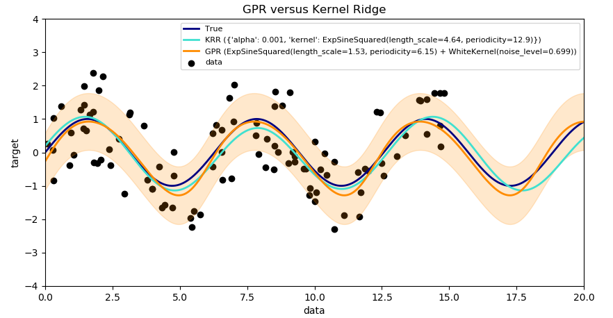
This example illustrates both methods on an artificial dataset, which consists of a sinusoidal target function and strong noise. The figure compares the learned model of KRR and GPR based on a ExpSineSquared kernel, which is suited for learning periodic functions. The kernel’s hyperparameters control the smoothness (l) and periodicity of the kernel (p). Moreover, the noise level of the data is learned explicitly by GPR by an additional WhiteKernel component in the kernel and by the regularization parameter alpha of KRR.
The figure shows that both methods learn reasonable models of the target function. GPR correctly identifies the periodicity of the function to be roughly 2pi (6.28), while KRR chooses the doubled periodicity 4pi. Besides that, GPR provides reasonable confidence bounds on the prediction which are not available for KRR. A major difference between the two methods is the time required for fitting and predicting: while fitting KRR is fast in principle, the grid-search for hyperparameter optimization scales exponentially with the number of hyperparameters (“curse of dimensionality”). The gradient-based optimization of the parameters in GPR does not suffer from this exponential scaling and is thus considerable faster on this example with 3-dimensional hyperparameter space. The time for predicting is similar; however, generating the variance of the predictive distribution of GPR takes considerable longer than just predicting the mean.